max(\(e^\pi\), \(\pi^e\))?
Greetings new blog readers and functional programming aficionados. The theme of the content here is rather varied so you’re unlikely to see any more functional programming articles for a while. Choosing the next topic for a new audience is crucial though and despite having a couple of ideas I decided to go with the mathematical / coding one. My experiences and advice on effective software development with team members thousands of miles away (told from my personal experience on both sides of the fence 😉 will have to wait until next week. Instead I’ll talk about a simple mathematical interview style puzzle. That I got wrong. And became a little obsessed over. Just a little.
A friend of mine who recently attended MathsJam tweeted about posing a small quantitative interview question. Which term is larger, \(e^{\pi}\) or \(\pi^{e}\)? Without giving away the answer I will state that it’s a tricky question to get right using mental arithmetic alone as one term is 97% of the other. And apparently with such little room for error, opinion over which term is the largest usually splits audiences roughly in half.
The main stumbling block I had with this puzzle was being unable to visualise how fractions affected powers. Too used to always having a calculator or coding window I didn’t know where to start. Sometimes visualising problems can be dangerous as an old theoretical physicist friend of mine once told me, “If you can visualise a 4 dimensional space, you’re doing it wrong” but I thought fractional powers was something that must be achievable. I was going to be playing around with a graphing library anyway for a quant library I’m writing (again, a blog post for another time) so here are the results of a wasted afternoon messing around with mathematics and WPF.
Interview Questions
The reason for tricky puzzles and obscure maths based questions in interviews often isn’t to know – or even work out – the answer, it’s about how you approach the problem and what conclusions and estimations you come to. Or whether you plain shrug your shoulders and give up… if that’s the kind of thing you do, you may have been talked about here.
Probably because my guess was wrong, I was determined to throw some completely over the top thinking at it to see if there was any way I could have done better. Before reading any further make your own guess now or think about how you’d go about solving it.
Rational Powers
I must admit I took a wrong turn when initially looking at this problem. With such small numbers as \(e\) and \(\pi\) which I could recall to the few required decimal places, calculating the two expressions seemed so tantalisingly close. Looking online for some help turned up this instructional YouTube clip, Evaluating Numbers Raised to Fractional Exponents. Seemed exactly what I needed, however there were two small problems. The numbers I’m dealing with are mathematical constants and not short, neat fractions. Of course, there are always estimations that can be made, \(3.141592\) is roughly \(\frac{31416}{10000}\) or at a push \(\frac{22}{7}\). But the main stumbling block with that video was the loaded examples i.e. \(4, 9, 16, 27\)… all well known powers of \(2\) and/or \(3\). Mentally working out the \(i\)-th root of a number isn’t an easier problem than calculating a fractional power to begin with. Perhaps I should have gone, as usual, straight to Wikipedia and their page on Exponentiation. Specifically the section on Real Exponents that helpfully actually defines what an expression with a real exponent is as well as presenting a handy way to compare rational exponents with the aid of a log table: \(b^x = e^{x.ln (b)}\). I quickly realised though that this line of thinking wasn’t helping me actually answer the question.
Calculus
Perhaps if I hadn’t seen the question posed via Twitter there may have been room to include an important bit of secondary information: you can easily work this out without a calculator. One of the first tools calculus gives you is the ability to sketch formulae by performing a few basic reasoning steps. For example, factor the function to find its roots; calculate the derivative of the function to find its maxima, minima and points of inflexion etc. But what functions do we have? None so far, but if we introduce unknowns into our expressions we can produce some. Let’s replace \(\pi\) from the puzzle with the variable \(x\). This gives us two functions:
\[ f(x) = e^x\]
\[ g(x) = x^e \]
Given \(f\) and \(g\) we can state the following, \(f(0) > g(0)\), \(f(e) = g(e)\) and \(f(100) > g(100)\) (or some other large number). The thing we actually want to know though is for \(x = \pi\), which is bigger? We should be able to work this out by concentrating on the point where the two functions \(f\) and \(g\) meet at \(x = e\). Functions meet in one of four ways. Given a point \(x\), two functions (f) and \(g\) such that \(f(x) = g(x)\) and \(h\), a number tending to zero:
\[f(x – h) > g(x – h), f(x + h) < g(x + h)\]
\[f(x – h) < g(x – h), f(x + h) > g(x + h)\]
\[f(x – h) > g(x – h), f(x + h) > g(x + h)\]
\[f(x – h) < g(x – h), f(x + h) < g(x + h)\]
The first two examples are where the functions cross over i.e. one is bigger than the other before point \(x\) and the reverse is true after. The latter two are where the functions touch but do not cross i.e. one function is bigger than the other before point \(x\) and after. Knowing which type of meeting \(f\) and \(g\) have will allow us to sketch them.
The type of meeting is governed by the gradients of the functions at point \(x\). If the gradients at point \(x\) are the same then the functions touch but don’t cross. If the gradient of function \(f\) at point (x) is smaller than the gradient of function \(g\) that implies that \(f\) was larger than \(g\) before point \(x\) and smaller after it.
So let us return to our definitions above, namely, \( f(x) = e^x \) and \( g(x) = x^e \). We can find their gradients by calculating their derivatives with respect to \(x\):
\[ f'(x) = \frac{d}{dx} e^x = e^x \]
\[ g'(x) = \frac{d}{dx} x^e = e.x^{e – 1} \]
The meeting point of \(f\) and \(g\) we want to sketch is \(x = e\). Lets compare gradients at that point.
\[ f'(e) = e^e \]
\[ g'(e) = e.e^{e – 1} = e^e \]
The gradients are the same which means \(f\) and \(g\) touch at \(x = e\) rather than cross. From earlier on above we also know that \(f\) is greater than \(g\) for larger and smaller values of \(x\). We can therefore produce the following sketch:
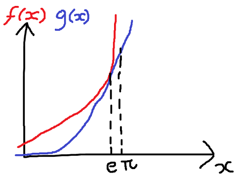
Sketch is maybe giving it more credit than its due but whatever. As you can see we want to know which function has the greater value for \(x = \pi\) and from this sketch it looks like that’s \(f\), therefore we can say that \( f(\pi) > g(\pi)\) or \(e^\pi > \pi^e\).
Another example
If you’re not sure you’ve completely got this lets work through another example. Thankfully we’ve got some expressions left over from which we can produce two different functions \(f\) and \(g\), namely:
\[ f(x) = \pi^x \]
\[ g(x) = x^\pi \]
Going through the list of things we know about these two functions we can state as before that \(f(0) > g(0)\), \(f(\pi) = g(\pi)\) and \(f(100) > g(100)\). Things look pretty similar to how they were before but we should expect that if our thinking from the last section was correct, \(f(e) < g(e)\). In order to sketch \(f\) and \(g\) we need to find their derivatives with respect to \(x\).
\[ f'(x) = \frac{d}{dx} \pi^x = ln(\pi).\pi^x \]
\[ g'(x) = \frac{d}{dx} x^\pi = \pi.x^{\pi – 1} \]
where \(ln(x)\) is the natural log of \(x\). Now compare the gradients of \(f\) and \(g\) at the point where they meet, \(x = \pi\):
\[ f'(\pi) = ln (\pi) . \pi^\pi \]
\[ g'(\pi) = \pi.\pi^{\pi – 1} = \pi^\pi \]
Cancelling out the common \(\pi^\pi\) term we can see that \( f'(\pi) = ln (\pi) . g'(\pi)\). We know that \(ln (e) = 1\) and because \( e < \pi \), \( ln (\pi) > 1 \), therefore \( f'(\pi) > g'(\pi) \). This means that when \(f\) and \(g\) meet at \(x = \pi\) they cross each other. \(f\) has a steeper gradient so is greater than \(g\) after \(x = \pi\) and smaller before then. Taking what we’ve learned, here is the sketch of \(f(x)\) and \(g(x)\).
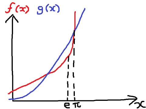
Without knowing where the other point at which \(f\) and \(g\) meet is, we can’t say with 100% certainty but it looks likely that \(f(e) < g(e)\), or more simply \(\pi^e < e^\pi\).
Graphing Tool
In refreshing myself with some basic calculus, and mainly because this blog is dedicated to implementing ideas, I decided to write a small function graphing app. To start with I used the excellent WPF Bezier Graphing Code Project by Ken Johnson. I also wanted to allow the user to specify their own functions. To that end I looked at the CSharpCodeProvider .Net class that allows strings containing code to be compiled dynamically at runtime. This compiled code can be used to produce executables or libraries but it can also be encapsulated on its own as an object and invoked, again dynamically, via reflection. I thought this was a neat yet powerful C++ style solution to the problem of letting the user specify a function. And by that I mean, “I’ve given the user plenty of rope, it’s their fault if they hang themselves with it.”
There is just one caveat with this tool, however. Bezier curves are fantastic at producing clear, smooth plots but require knowledge of the derivative of the function as well as the function itself. This means unless you have some knowledge of calculus yourself (and I’m guessing if you’ve read this far you do) or you’re plotting complex functions, this may not be the appropriate tool for you. That said, there are always helpful places you can go to for differentiating functions.
To get the ball rolling then, here are the two sketches from above recreated with the aid of my graphing tool:
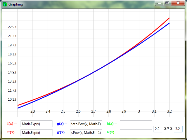
\[ f(x) = e^x, g(x) = x^e \]
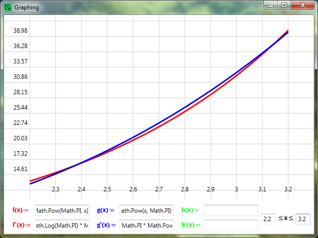
\[ f(x) = \pi^x, g(x) = x^\pi \]
Using the Graphing Tool
As the text boxes don’t show the functions fully, here are the definitions for the latter example where \(f(x) = \pi^x\) and \(g(x) = x^\pi\):
Math.Pow(Math.PI, x)Math.Log(Math.PI) * Math.Pow(Math.PI, x)Math.Pow(x, Math.PI)Math.PI * Math.Pow(x, Math.PI - 1)
As you can these, the user is welcome to use any of the functions in the Math namespace. But more than that you can enter any legal C# code constructs. The string you write is simply being dropped into this line of code:
Func<double, double> function = x => *YourStringHere*;
The executable and GPL source code and project files can be found in the Download section. Have fun 😉