Helping a stranger (and why you should understand NP-complete)
Earlier this year I helped out a random Hacker News commenter. This was covered in a recent blog post where I discussed the trade off between being an expert or a generalist. Realising my GitHub repository was littered with short, generalist introductions and experiments, I concluded that I should add the complex NP-complete constraint solver I had been working on for the past few years – an area in which I had some expertise.
At least, I thought that was the conclusion.
Help comes at a great cost, you must first ask for it
Hacker News isn’t just about start ups. I’m always amazed that however obscure the subject area there are industry experts who start discussing the finer technical aspects of a given post. Another pattern I love about the comments and community is how readily people want to network by reaching out a helping hand e.g. “If you’re interested in XYZ, drop me an email. I can provide more details.”
It takes a rather specific situation to be able to offer help however. You have to be knowledgeable about a domain that can’t easily be simplified by series of web searches, and more importantly, there has to be a suggestion that someone might be seeking that clarification. In spite of everything any one person might know, this situation doesn’t occur frequently.
My story about helping a stranger started with a Hacker News post about a programmer who had solved an NP-complete problem from an xkcd strip using the constraint solver, MiniZinc.
The comments section turned into a mini-debate about the nature of the problem and combinatorial problems in general. Put simply, combinatorial problems are those that require the enumeration of combinations of possible choices. The archetypal problem in this area is the Travelling Salesperson: given a set of cities to visit represented as a weighted graph, find the shortest route that takes the traveller from his or her starting node (city) around all the other nodes in the graph and returns them back to the start. Finding a solution to this problem is a known computationally hard problem and requires several different sub-paths through the graph to be tried again and again in combination with others.
One particular commenter described a problem he had which he knew was combinatorial in nature but was part of a low-level device driver written in C. As such, the available open source techniques like Prolog or even the 3rd party C++ device drivers were too heavy-weight for his particular use case. Without having the relevant domain knowledge for solving combinatorial problems, he had hard coded a bruteforce algorithm to enumerate all the combinations but was looking for help to solve the problem more efficiently: “…I really don’t know where to start. Any pointers/things to google for?”
So here it was, an area in which I felt I had a significant amount of knowledge, and an unequivocal request for assistance. Even though I’m always busy and time is at a constant premium, I somehow thought offering it for free was the right thing to do.
The Problem
My offer of help was accepted and I was introduced to the problem of Phase Locked Loops. Given an input frequency and a desired output frequency, choose values for the integers \(f\) and \(r\), and the power of 2, \(q\), that satisfies the following equation:
\[output = \frac{input.f}{r.q}\]
This could be solved in an acceptable amount of time with a brute force search, but the actual problem which the request for help concerned was the serial placement of two phase locked loops which increases the complexity by a significant amount. The output of the first PLL circuit becomes the input frequency of the next.
\[output = \frac{tmp.f2}{r2.q2}\]
\[tmp = \frac{input.f1}{r1.q1}\]
Finding the values for \(f1\), \(r1\) and \(q1\) requires simultaneously searching the possible combinations of \(f2\), \(r2\), \(q2\). Thus, the complexity of the problem.
A bruteforce enumeration can be achieved using a six levels deep nested for loop.
for (int r1 = 1; r1 < = 64; ++r1)
  for (int f1 = 1; f1 <= 256; ++f1)
    for (int q1 = 1; q1 <= 256; q1 <<= 1)
      for (int r2 = 1; r2 <= 64; ++r2)
        for (int f2 = 1; f2 <= 256; ++f2)
          for (int q2 = 1; q2 <= 256; q2 <<= 1)
            if (output * r1 * r2 * q1 * q2 == input * f1 * f2)
            {
              sol->f1 = f1;
              sol->f2 = f2;
              sol->r1 = r1;
              sol->r2 = r2;
              sol->q1 = q1;
              sol->q2 = q2;

              return 1;
            }
At the heart of the deepest level is a check to see if the values satisfy the above formula. By considering the bounds of this problem i.e. the range of valid values for each unknown, we can calculate the number of possible combinations. The \(f\) variables can be between 1 and 256, the \(r\) variables between 1 and 64 and the \(q\) powers of 2 can be from 1 to 256, so there are eight potential values. This leads to a total of \(256^2.64^2.8^2\), or \(17,179,869,184\) – a staggering number of combinations to enumerate in a device driver.
By taking a few of the techniques from the discipline of constraint solving, it’s possible to cut down drastically the number of combinations to consider. Before that though, let’s take a digression through complexity theory and, more specifically, P, NP and NP-completeness.
Understanding NP-complete completely useless?
The concept of NP-completeness was introduced in the early seventies by mathematician Stephen Cook. The question of whether an NP-complete problem could be solved deterministically in polynomial time, essentially is P=NP a true statement, has been an open question ever since – one whose answer is worth $1m.
I’ve heard some Computer Science lecturers glaze over at the term “NP-complete”. It’s one of those theoretical concepts like, say, finite automata, that unless you deal with on a daily basis, it’s easy to completely forget. More worringly it’s easy to assume it’s not important.
Most good programmers have a solid grasp of Big-O notation. They can tell you that the most efficient algorithm for ordering (randomised) data is Quicksort, which has a Big-O notation of \(O(n \log n)\). This is preferable to Bubblesort which has a Big-O notation of \(O(n^2)\). However, in terms of Complexity Theory, these algorithms are two peas in the same pod in that they’re both members of the classification of problems denoted by P.
P in this case stands for polynomial – the amount of space and time required for these algorithms to complete can be represented as polynomial functions of the size of the input. Higher order polynomials may make a program less responsive, or require more memory, but generally speaking they are still tractable (solvable) problems.
There are many complexity classes and the relationships between them are, suitably enough, quite complex. One of the first that is introduced to those learning about complexity theory is NP. Not “Non-Polynomial” as many incorrectly recall, but “Non-deterministic Polynomial”. The distinction is subtle but important.
This complexity class is a superset of P i.e. every problem in P is also in NP. For a problem to be classified as Non-deterministic Polynomial, it similarly requires that a solution to the problem can be found within polynomial time. However, rather than running on a computer that behaves predictably and is Turing-complete, we can use a non-deterministic Turing machine. Such a machine behaves unpredictably. Whereas a deterministic algorithm performs each instruction predictably one after the other, a non-deterministic machine can at any point in the program have multiple instructions to follow and it chooses which one to execute non-deterministically. If a polynomial time algorithm can be written where it’s possible that the correct instructions will be executed and a solution found, then that problem is said to be in the complexity class Non-deterministic Polynomial.
Though every problem in P is in NP, the relationship between P, NP and NP-complete is not so well known. The definition of NP-complete, though oft misunderstood, requires only two conditions to be met. A problem \(Z\) is NP-complete if:
- Every problem in NP can be polynomial time reduced i.e. mapped, to \(Z\)
- The output of the algorithm solving \(Z\), known as a token or certificate, can be verified as a valid solution in polynomial time
That first condition looks quite daunting. For a problem to be NP-complete it needs to be proved that it can be reduced to every other problem in NP!? Thankfully no, the Cook-Levin Theorem goes through the tough work of showing that the Boolean Satisfiability problem, commonly known as SAT, is NP-complete. Now we can take a shortcut to satisfying point 1 above by showing a problem is polynomial time reduceable to another NP-complete problem.
Indeed, some of the most cutting edge combinatorial problem solving techniques still exist in specifying a problem as a SAT instance. And this is the crux of the problem with combinatorial problems, they’re NP-complete and take a long time to solve. Whether P is actually equal to NP or not is in some ways irrelevant because for now they are separate entities. NP-complete is essentially shorthand for belonging to a class of problems that are computationally very hard i.e. there are no known general purpose polynomial time algorithms for them.
For those brave souls who’ve read all of this digression, you might be asking, “Isn’t this just logical navel gazing? What on earth is useful about knowing these theoretical class relationships?”
Good judgement in selecting the correct abstract data type (ADT) for collections in your code is the type of decision that programmers commonly make. Have a large collection of constant data that requires frequent, randomised access? Use a vector / array. A collection of ordered elements continuously being added to and removed from? AVL or Red-Black tree. Most programmers don’t write their own implementations of these algorithms but rely on library providers. What’s important is that they understand what the underlying Big-O notation is for each of the different operations (add, remove, access, iterate) of each ADT and thus choose the correct one. The application of understanding NP-completeness though much a rarer event is crucial for being an expert coder.
But in the style of Mr Miagi, I’ll defer the why until later. My apologies 😉
How to solve combinatorial problems
Back to the task at hand. Given a combinatorial problem that consists of \(n\) unknowns, that each have \(d\) possible values, and must satisfy one or more properties, how best are we to solve this mammoth task? First of all, understand that the Big-O notation for bruteforce enumeration of the combinations that exist in this problem is \(O(d^n)\). If \(d\) and \(n\) are double-digit numbers it’s likely that this naive implementation cannot be relied upon.
Given that there is an exponential number of possibilities there are two main approaches. In the first case, if the problem is well understood there may be optimal algorithms with acceptable efficiency, for instance graph colouring is one such problem. For lesser known or less generic problems, there are common strategies that can be applied that will greatly reduce the worst case \(O(d^n)\).
1. One choice at a time
Instead of considering a full combination of choices for each unknown and testing whether all the conditions are satisfied, take one choice at a time and test whether any one of the conditions is inconsistent. Or to put it another way, consider the naive enumeration of the full combinations to be a breadth first search at the lowest level of a tree, n nodes deep with d children at each node (remember, \(d^n\) combinations).

We want to consider choosing a value for just the first unknown to begin with then looking to see if there are any inconsistencies. To take PLL as an example, the first choice would be \(f1=1\). As yet, there are no apparent inconsistencies so we continue to traverse the search space until we do. By employing a depth-first search we can (a) navigate the entire exponential search space using just \(O(d.n)\) memory and (b) we can backtrack from any node with inconsistencies and thus avoid enumerating the children nodes of that subtree. For example, in the above diagram consider \(v1=2\), marked in purple, to be an invalid state. We can automatically rule out all the child nodes in the tree and save exploration of one third of all full enumerable states.
2. Inference
If we have a condition that says an unknown \(a\) must be less than \(b\), and the node in the search tree we’re currently at has chosen \(a\) to be 5, we can reason that \(b\) must be at least 6. We now no longer have to consider \(b\) equal to 1, 2 or 3 etc. This is because we understand the semantics of the binary less-than operator. The great benefit of these removals is that each one itself is the root node of an exponential subtree. Any polynomial computation performed in finding inconsistent states ahead of time will likely be worth it in the long run.
3. Heuristics
The instantiation of the unknowns can be done in any order. An algorithm for choosing which unknown to consider next is called a heuristic, and it can make a big difference to solving the problem. It sounds counter intuitive but if we have 5 unknowns that have a large number of possible values, but one unknown with only 3 possible values remaining, we should choose to instantiate the unknown with the smallest number of possible values. That’s because with only three subtrees to consider we will find either a solution, or lack of one, sooner than we would by instantiating the unknowns with a large number of subtrees. Even if we don’t find a solution that’s still good because it means we get to backtrack higher up the tree thus ruling out more of the search space. This ploy of tackling the part of the search space that looks most likely to yield no solution is called “Fail First”.
In quickly blasting through the above, I’ve left out a lot of other potential general purpose techniques and glossed over some of the detail. If any of it has piqued your interest, however, I recommend having a look at constraint programming or constraint logic programming. You haven’t truly beaten Sudoku until you’ve written a program to solve them.
Encoding PLL as a CSP
Constraint programming is the discipline of solving Constraint Satisfaction Problems (CSPs) – these are general purpose combinatorial problems consisting of a simple model with unknowns (variables) each with range of potential values (domain) and rules on what constitutes a valid solutions (constraints). Once the model and constraints have been specified it suffices for the constraint solver to traverse the search space using the techniques described in the previous section.
Before I attempted to help create a specialised algorithm in C for solving the PLL problem, I constructed it as a CSP for my own favourite constraint solver – the one I’ve been writing in C# on and off for the last few years. By coding it as a CSP and experimenting with the heuristics and constraints, I hoped to get a better feel for where the big gains in efficiency might come from.
It had been a while since I’d worked on my constraint solver – over a year. I used to be a constraint programming researcher and even though I had no specific skills in performance critical systems, I knew the style of expressive, easy to use syntax I wanted for specifying constraints. I had a concise variable representation and solid arithmetic propagation algorithms. And yet, if it weren’t for this exercise how much longer would it have been sat gathering dust helping no-one?
As well as the central constraints represented as two connected formulae shown in The Problem section, there were valid ranges for certain frequency bounds. For example, \(10 \leq \frac{input}{r1} \leq 1000\). These are fantastic constraints because they have what’s know as a small arity i.e. the constraint acts on a small number of variables. More often than not, this makes for better propagation than one that acts on several.
Encoding the additional inequality constraints led to a quick succession of NotImplemented exceptions being thrown. I had writen propagators for every overrideable binary operator in C# apart from the inequality operators. An afternoon of work later and I had a much improved PLL solver as well as a more complete constraint solver. I examined the code and performed a few of ReSharper’s saner suggested changes.
It all felt like such a waste of my work. This solver was going to be the pivotal element in my grand cloud based planning and scheduling venture. And yet, I knew giving that startup idea a go was way down my list of priorities – it wasn’t even my number one startup idea. Perhaps it was time to share what I’d spent so many evenings and weekends on with the world. What did I have to lose?
I added my solver, named Decider, to my GitHub repository along with a few example CSPs implementations, notably, Phase Locked Loops.
Solving an NP-complete problem in a C driver
When writing a low-level hardware driver in C, being responsive is paramount. One commenter in the original Hacker News thread said, “an algorithm with performance bounds tight enough that you can use it in a device driver — probably doesn’t exist … the fact that you’ve resorted to brute force search to this point suggests there may not be.” And to be honest, I agree. But for such a specific problem we can take a hacker’s approach and implement just enough to be performant without writing a low level constraint solver in C.
As briefly discussed above, arithmetic constraints are useful because the binary operators propagate well. Given a[1..5], b[1..5] and c[1..100] and the constraint a + b = c, we can infer a reduced set of bounds for c, [2..10]. Constructing propagators for the multiplication and equality operators (those found in the implied constraint for the PLL problem \(output.r1.r2.q1.q2 = input.f1.f2\)) is fairly straightforward. The difficulty comes however in constructing a system to update bounds dynamically at each node during a depth-first search tree traversal – that we incidentally have also not yet written.
Though the arithmetic constraint is useful, a much simpler optimisation came from collectively analysing the inequality constraints. Together, they dictate constantly altering upper and lower bounds for the values of each of the six unknowns. Upper and lower bounds that can be easily set in a for loop.
\[25 \leq input \leq 600\]
\[10 \leq \frac{input}{r} \leq 1000\]
\[1600 \leq \frac{input.f}{r} \leq 3200\]
In the end, the change required was subtle, and yet effective.
for (int r1 = input / 1000 + 1; r1 < = input / 10; ++r1)
  for (int f1 = (1600 * r1) / input + 1; f1 <= (3200 * r1) / input; ++f1)
    for (int q1 = 1; q1 <= (input * f1) / (25 * r1); q1 <<= 1)
      for (int r2 = (input * f1) / (r1 * q1 * 1000) + 1; r2 <= (input * f1) / (r1 * q1 * 10); ++r2)
        for (int f2 = (1600 * r2 * r1 * q1) / (input * f1) + 1; f2 <= (3200 * r2 * r1 * q1) / (input * f1); ++f2)
          for (int q2 = 1; q2 <= 256; q2 <<= 1)
            if (output * r1 * r2 * q1 * q2 == input * f1 * f2)
            {
              sol->f1 = f1;
              sol->f2 = f2;
              sol->r1 = r1;
              sol->r2 = r2;
              sol->q1 = q1;
              sol->q2 = q2;

              return 1;
            }
We can consider each inner block as a further step into the search space with all the upper nodes bound to values. As such we can use the inequalities to act as propagation constraints to reduce the bounds of the next variables. Gaining as many prunes to the search space as this for such a small change was surprising but welcome.
Recognising NP-complete problems
The request for help came to me from someone who had already realised the most crucial detail of the problem in question. That the naive, combinatorial enumeration used in solving it suggested an NP-complete problem.
Bubblesort, the \(O(n^2)\) implementation of sorting is bad. Inserting into or searching from an array carries a \(O(n)\) penality which implies the wrong data structure is being used. Perhaps an ill thought out needless repetition turns a \(O(n^3)\) operation into a \(O(n^5)\)? These are all bad inefficiencies and poor programming. But they are nothing in comparison to an NP-complete problem.
When we’re introduced to concept of Big-O notation, it usually accompanies a graph such as this. The \(n \log n\) is preferable because it grows slower than the rest, and the exponential \(1.1^n\) term should be avoided.
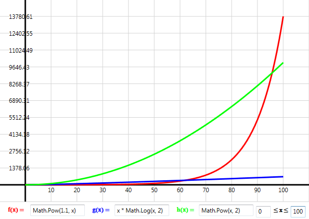
I remarked earlier that polynomial problems are like peas in a pod compared to NP-complete problems. An exponential function viewed close up as above doesn’t look too different to the other polynomial curves. The true scale of the exponential isn’t appreciated until we step back. (These graphs were created using this open source Windows graphing tool).
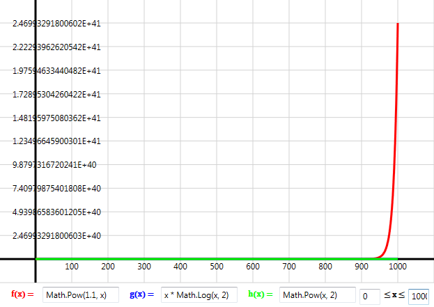
Problems in P, even badly encoded ones, have gradual runtime increases with respect to larger inputs. NP-complete problems on the other hand, go from being, fast or responsive to time consuming, to painfully slow, to unsolvable in a year – all in the space of an ever so slightly increased problem size. Think of NP-complete problems as if they were a brick wall like the red plot in the above graph. Understanding the theory behind the NP-complete complexity class means recognising intractable problems in your code – it’s like having a bomb sniffer dog when walking through a minefield. If you can map your problem to, say, graph homomorphism, or any other NP-complete problem, you know for sure, 100% guaranteed that this will not be an easy problem to solve. Thus at the very least it will need a specialised approach, or possibly it should be discarded altogether.
They are rare, but I recently spotted one at work in a complex regulatory software solution for generating LSMC proxy functions for Solvency II. What surprised me the most after I looked into it was that firstly, no-one else had realised it was an NP-complete problem but rather just thought it was an inefficient bit of code. But more dangerously, even though it was known to be inefficient, I don’t think the seriousness was grasped of what it means to have an NP-complete problem in your code.
If I hadn’t helped that stranger, I wouldn’t have updated and tidied up my solver, I wouldn’t have made it available on GitHub, there wouldn’t have been a chance I could quickly solve this problem. But because I did, I had an open source project ready to go – by helping another, I’d helped myself!
What being helpful (and understanding NP-complete) got me
Using a 3rd party open source library requires some bureaucratic dotting of “i”s and crossing of “t”s such is the bloat in a large software house. The legal department thankfully made a small concession in signing off my licence terms. Though I’m a software developer, I work for the product management team and as such I get a bit of stick for not being a true dev, but the main complaint is that I eat “developer” cakes. As someone who needs to be on the development team mailing list for serious, work related reasons, I am happily also privvy to the frequent notifications regarding the availability of cakes around the developer desks. As I go by and help myself to a cookie, doughnut or muffin, I’m occasionally challenged by the head of the team, “What are you doing? Those aren’t for you.”
It pleased me greatly that my MIT licence was included along with my 3rd party library and that the IP Report for this big ticket enterprise software recognises my entitlement to cake.
TL;DR? I helped a stranger on Hacker News and as a direct result I was able to use my constraint programming library I’d been working on for some years in an important software product at work.
I have no idea what the stranger’s project was other than something to do with a video codec. More importantly, I can image a dozen different ways in which I could help someone out and nothing good would come back to me. However, I would never have predicted how fortuitously the timing worked out for me in this case. For those who find themselves in a similar position in future, if you have the time, expertise and energy: help out a stranger – you never know where it might lead.